2. Evaluating Memory Models

Funding and Authorship

This post was made possible by research funding generously provided by AnkiHub and was written in collaboration with Giacomo Randazzo.

Comments

This text is also available on AnkiHub’s Forum (link coming soon). For comments and discussion, please go there.

---

In a previous post, we introduced the concept of a memory model as a function that takes a student, their review history, and a card, and returns a forgetting curve that gives the retrievability of the card as a function of time. In this post, we discuss how we might evaluate and compare memory models, in particular we’ll motivate our choice of metrics:

• Normalized Entropy (Normalized Log Loss)
• Brier Skill Score (Normalized Brier Score)
• SmoothECE (and calibration plot)
• AUC (and ROC curve)
• All 8 Major Confusion Matrix Statistics at prediction thresholds $\tau \in \{0.85,0.9,0.95\}$
• Temporal Discrimination Check

Our goal is that this post will serve as a clear and accessible introduction for developers and researchers interested in memory models for spaced repetition. We hope you come away with an improved understanding of what each of the metrics means and why we chose it. We’ve chosen to err on the side of covering things in detail, and explaining concepts we expect readers might not already be familiar with. We assume you’re familiar with probability theory, but not with information theory or machine learning.

A note on scope: we discuss these metrics in the context of model evaluation and comparison, not as training objectives. We are asking ‘which model is better?’, not ‘what should we optimize during training?’ The choice of objective function is largely decoupled from comparison metrics — the metrics we propose here can be used to compare memory models trained on a diversity of objectives. What metric to hill-climb on during training is a separate engineering question involving model-specific concerns like regularization.

Proper Scoring Rules

A memory model is a kind of forecaster, something that makes predictions about outcomes. A scoring rule is a function that we can use to evaluate forecasters. It takes their prediction, along with the actual outcome, and outputs a number representing the quality of the forecast.

Sebastian Nowozin has written a helpful blog post which I have edited slightly to improve readability within the context of this article:

Given a set of possible outcomes $\mathcal{Y}$ and a class of probability measures $\mathcal{P}$ defined on a suitably constructed $\sigma$-algebra, we consider a forecaster which makes a forecast in the form of a probability distribution $P\in \mathcal{P}$. After the forecast is fixed, a realization $y\in \mathcal{Y}$ is revealed and we would like to assess quality of the prediction made by the forecaster.

A scoring rule is a function $S$ such that $S(P,y)$ is taken to mean the quality of the forecast. Hence the function has the form $S:\mathcal{P}\times \mathcal{Y}\to \mathbb{R}\cup \{-\infty ,\infty \}$. There are two variants popular in the literature: the positively-oriented scoring rules assign higher values to better forecasts, the negatively-oriented scoring rules behave like loss functions, taking smaller values for better forecasts.

A proper scoring rule has desirable behavior, to be made precise shortly. Let us think what could be desirable in a scoring rule. Intuitively we would like to make “cheating” difficult, that is, if we really subjectively believe the forecast $Q\in \mathcal{P}$, we should have no incentive to report any deviation from $Q$ in order to achieve a better score. Formally, we first define the expected score under distribution $Q$ when reporting a forecast $P$

$$S(P,Q)={\mathbb{E}}_{y\sim Q}[S(P,y)]$$

So that if we believe in any prediction $Q\in \mathcal{P}$, then we should demand that (for negatively-oriented scores)

$$S(Q,Q)\le S(P,Q),\forall P,Q\in \mathcal{P}$$

For strictly proper scoring rules the above inequality holds strictly except for $Q=P$. For a proper scoring rule the above inequality means that in expectation the lowest possible score can be achieved by faithfully reporting our true beliefs. Therefore, a rational forecaster who aims to minimize expected score (loss) is going to report his beliefs.

It is desirable that the scoring rules we use to evaluate memory models are proper, because it ensures the models are incentivized to do the best that they can, rather than reporting something other than what they believe simply to game the metric. For example, under the improper scoring rule $S(p,y)=|p-y|$, the model is incentivized to always predict $p=1$ or $p=0$ to minimize its loss. Our set of metrics includes two proper scoring rules: the log loss, and the Brier score.

Actually, we use normalized versions of these scores to facilitate model comparison when the models are trained on different datasets, but this is a technical detail you can ignore for now until we discuss it later in the post.

The Log Loss (aka Binary Cross Entropy Loss)

Throughout this article, we will use the convention of negatively-oriented scoring rules. Meaning the output of $S$ is always $\ge 0$ and lower is better. Technically, the Log Loss we discuss throughout is the Negative Log Loss, though that loss is commonly referred to as simply the Log Loss throughout the ML literature. We will remain consistent with that convention.

For a prediction $p\in (0,1)$ and outcome $y\in \{0,1\}$, the (negative) log loss scoring rule for probabilistic binary classification is given by

$$S(\text{Bernoulli}(p),y)=-y\ln (p)-(1-y)\ln (1-p)$$

For a dataset of $N$ reviews, typically we report the mean log loss across examples:

$$\frac{1}{N}\sum _{i=1}^{N}S(\text{Bernoulli}(p_i),y_i)$$

where $p_i$ is the prediction of the model for the $i$-th example.

Proof: the log loss for probabilistic binary classification is strictly proper

Recall that a scoring rule is strictly proper if and only if $S(P,Q)$ is uniquely minimized when $P=Q$.

In the case of probabilistic binary classification, $P$ and $Q$ are Bernoulli distributions parameterized by a single probability each, which we will call $p$ and $q$ respectively. Note $q$ is the prediction the forecaster believes to be true, while $p$ is the belief they report.

Additionally recall that, $S(P,Q)={\mathbb{E}}_{y\sim Q}[S(P,y)]$, so in the binary case

$$S(\text{Bernoulli}(p),\text{Bernoulli}(q))={\mathbb{E}}_{y\sim \text{Bernoulli}(q)}[S(\text{Bernoulli}(p),y)]$$

Since the expected value of $y$ is $q$ in the opinion of the forecaster, the forecaster’s expectation ${\mathbb{E}}_{y\sim \text{Bernoulli}(q)}[S(\text{Bernoulli}(p),y)]$ is given by

$${\mathbb{E}}_{y\sim \text{Bernoulli}(q)}[S(\text{Bernoulli}(p),y)]=-q\ln (p)-(1-q)\ln (1-p)$$

Now, we wish to know the value of the stated prediction $p$ relative to the believed prediction $q$ that minimizes ${\mathbb{E}}_{y\sim \text{Bernoulli}(q)}[S(\text{Bernoulli}(p),y)]$. So we evaluate the derivative of ${\mathbb{E}}_{y\sim \text{Bernoulli}(q)}[S(\text{Bernoulli}(p),y)]$ with respect to $p$, equate it with 0, and solve.

$$\frac{d{\mathbb{E}}_{y\sim \text{Bernoulli}(q)}[S(\text{Bernoulli}(p),y)]}{dp}=-\frac{q}{p}+\frac{1-q}{1-p}=0$$ $$q(1-p)=p(1-q)$$ $$q-qp=p-qp$$ $$q=p$$

Finally, we verify that $p=q$ is a minimum and not a maximum or saddle point. We evaluate the second derivative of ${\mathbb{E}}_{y\sim \text{Bernoulli}(q)}[S(\text{Bernoulli}(p),y)]$ with respect to $p$:

$$\frac{d^2{\mathbb{E}}_{y\sim \text{Bernoulli}(q)}[S(\text{Bernoulli}(p),y)]}{d{p}^2}=\frac{q}{p^2}+\frac{1-q}{(1-p{)}^2}$$

Since $q\in (0,1)$, both terms are strictly positive for all $p\in (0,1)$. Therefore ${\mathbb{E}}_{y\sim \text{Bernoulli}(q)}[S(\text{Bernoulli}(p),y)]$ is strictly convex in $p$, and the unique critical point $p=q$ is a strict global minimum. So the forecaster minimizes their expected loss uniquely by reporting their true belief, therefore the log loss is strictly proper.

The information theoretic interpretation of the log loss.

The log loss has a useful and beautiful information theoretic formulation, but to understand it, you first need to be acquainted with the definitions of entropy and KL divergence in information theory, at least as they pertain to a Bernoulli distribution.

Entropy

The entropy of a discrete probability distribution (for instance a Bernoulli distribution) is, informally speaking, a measure of how “random” it is. It is the expected surprise you experience when you sample from the distribution. For a discrete random variable $X$ with possible outcomes $\{x_1,\dots ,x_J\}$ and probability distribution $Q$ where $Q(x_j)=q_j$, the entropy is:

$$H(Q)={\mathbb{E}}_{X\sim Q}[-\ln (Q(X))]=-\sum _{j=1}^J{q}_j\ln (q_j)$$

The $-\ln (q_j)$ term represents the surprise of outcome $j$. The smaller $q_j$, the more you’re surprised when you observe $x_j$. In the limit as the outcome becomes more and more rarefied, you approach infinite surprise. But why do we use a negative logarithm to represent surprise? You’re increasingly surprised the more unsuspected an event, therefore we want it to be large for small probabilities. That’s why we use the negative log instead of the log, so we get a large positive number for probabilities approaching zero. If three independent rare events happen you will be three times as surprised, compared to just one of them happening, since probabilities of independent events multiply, and we want surprise to add, the logarithm is the only continuous function we can choose (${\log }_x(a)+{\log }_x(b)={\log }_x(a\cdot b),\forall x\in {\mathbb{R}}^{+}\setminus \{1\},\forall a,b\in {\mathbb{R}}^{+}$). Conversely, when something we expect to happen happens, we aren’t very surprised at all, which matches the behavior of logarithms, which approach $0$ as their argument approaches $1$.

The entropy is maximized when $Q$ is uniform and minimized when $Q$ places all its probability mass on a single outcome. The maximum is unbounded above in general, but for a given $J$ is bounded above by $-{\sum }_{j=1}^J\frac{1}{J}\ln \frac{1}{J}=\ln (J)$. The smallest possible entropy is 0.

The entropy of a Bernoulli distribution ($J=2$) parameterized by $q$ is

$$-q\ln (q)-(1-q)\ln (1-q)$$

You will notice this is maximized at $q=0.5$, which is in some sense the “most random” Bernoulli distribution.

KL Divergence (aka Relative Entropy)

The KL divergence (Kullback-Leibler divergence), also called the relative entropy, is a measure of how much one probability distribution diverges from another. In Bayesian terms, the KL divergence $D_{\text{KL}}(Q\Vert P)$ is the extra surprise that an agent who believes $Q$ expects you to experience because you believe $P$.

For a discrete random variable $X$ with possible outcomes $(x_1,\dots ,x_J)$ and two probability distributions $Q$ and $P$ over those outcomes, the KL divergence from $Q$ to $P$ is:

$$D_{\text{KL}}(Q\Vert P)=\sum _{j=1}^J{q}_j\ln \frac{q_j}{p_j}$$

To see why this is the “extra surprise”: recall that $-\ln (p_j)$ is the surprise you experience when you observe outcome $y_j$ and you believe the distribution is $P$. Meanwhile $-\ln (q_j)$ is the surprise an agent who believes $Q$ experiences for the same outcome. Suppose such an agent knows you believe $P$. The agent’s expectation of your total surprise is

$${\mathbb{E}}_{X\sim Q}[-\ln (P(X))]=-\sum _{j=1}^J{q}_j\ln (p_j)$$

which we can decompose by adding and subtracting $q_j\ln (q_j)$:

$$-\sum _{j=1}^J{q}_j\ln (p_j)=-\sum _{j=1}^J{q}_j\ln (q_j)+\sum _{j=1}^J{q}_j\ln (q_j)-\sum _{j=1}^J{q}_j\ln (p_j)$$ $$=\underset{H(Q)}{\underbrace{-\sum _{j=1}^J{q}_j\ln (q_j)}}+\underset{D_{\text{KL}}(Q\Vert P)}{\underbrace{\sum _{j=1}^J{q}_j\ln \frac{q_j}{p_j}}}$$

So the agent expects you to incur a loss equal to the entropy $H(Q)$ — the surprise the agent themselves would experience — plus the KL divergence, which is the extra surprise the agent expects you to suffer because you believe and report $P$ instead of $Q$. The KL divergence is the expected value of this per-outcome excess surprise $\ln \frac{q_j}{p_j}$ under the agent’s belief $Q$.

Some properties:

• $D_{\text{KL}}(Q\Vert P)\ge 0$ always, with equality if and only if $P=Q$. You believe that $Q$ is more correct, so you always expect someone who believes $P\ne Q$ to be more surprised than you are. This is called Gibbs’ Inequality.
• $D_{\text{KL}}(Q\Vert P)$ is not symmetric: It is not in general the case that $D_{\text{KL}}(Q\Vert P)=D_{\text{KL}}(P\Vert Q)$. So KL divergence is not a metric, though it is used as a notion of “distance” between distributions.
• $D_{\text{KL}}(Q\Vert P)$ is undefined if there exists any outcome $y_j$ such that $q_j>0$ and $p_j=0$. If I think something can happen, and you say it’s infinitely impossible ($p=0$) then I think you’re infinitely wrong and say ‘to hell with the KL divergence!’

The KL divergence of a Bernoulli distribution $\text{Bernoulli}(p)$ from a Bernoulli distribution $\text{Bernoulli}(q)$ is

$$D_{\text{KL}}(\text{Bernoulli}(q)\Vert \text{Bernoulli}(p))=q\ln \frac{q}{p}+(1-q)\ln \frac{1-q}{1-p}$$

The log loss decomposes into entropy plus KL divergence

Now we can make the connection between information theory and the log loss for probabilistic binary classification. Recall that our expected log loss when the forecaster reports $p$ but we believe $q$ is

$${\mathbb{E}}_{y\sim \text{Bernoulli}(q)}[S(\text{Bernoulli}(p),y)]=-q\ln (p)-(1-q)\ln (1-p)$$

This decomposes into the entropy of $\text{Bernoulli}(q)$ plus the KL divergence of $\text{Bernoulli}(p)$ from $\text{Bernoulli}(q)$.

Proof that the expected log loss decomposes into the entropy of our belief and the KL divergence of the forecaster's belief from our belief

We want to show that the expected log loss for a prediction $p$ from the perspective of an agent who believes $q$ is given by

$$H(\text{Bernoulli}(q))+D_{\text{KL}}(\text{Bernoulli}(q)\Vert \text{Bernoulli}(p))$$

Simply expanding the definitions, we have

$$=\left[-q\ln (q)-(1-q)\ln (1-q)\right]+\left[q\ln \frac{q}{p}+(1-q)\ln \frac{1-q}{1-p}\right]$$

Then, expanding the log quotients:

$$=-q\ln (q)-(1-q)\ln (1-q)+q\ln (q)-q\ln (p)+(1-q)\ln (1-q)-(1-q)\ln (1-p)$$

The $q\ln (q)$ terms cancel, and the $(1-q)\ln (1-q)$ terms cancel, so we’re left with

$$=-q\ln (p)-(1-q)\ln (1-p)$$

Which is exactly ${\mathbb{E}}_{y\sim \text{Bernoulli}(q)}[S(\text{Bernoulli}(p),y)]$.

So the log loss we expect a forecaster with forecast $p$ to incur when we believe $q$ is the sum of the entropy of our belief $H(\text{Bernoulli}(q))$ (the surprise we ourselves would experience) plus the KL divergence $D_{\text{KL}}(\text{Bernoulli}(q)\Vert \text{Bernoulli}(p))$ (the extra surprise we expect the forecaster to suffer because they believe $P$ instead of $Q$).

Since $D_{\text{KL}}(Q\Vert P)\ge 0$ with equality if and only if $P=Q$, this gives us another way to see that the log loss is strictly proper: the forecaster minimizes their expected loss exactly when their prediction matches their belief, and the minimum achievable expected loss in their opinion is the entropy of their belief.

Is the log loss the cross entropy? Intro to the mind projection fallacy.

It’s quite common to hear the log loss called the cross entropy loss. This is because the log loss and the cross entropy share a functional form. So, it’s important to realize that many people use “cross entropy loss” to refer to log loss. However, conflating them confuses several distinct concepts that we think it is better to track independently, at least in your own head.

Specifically, we can consider four distinct quantities:

1. The per-sample log loss. Given a forecaster’s prediction $p_i$ and a realized outcome $y_i\in \{0,1\}$, the log loss is

$$S(p_i,y_i)=-y_i\ln (p_i)-(1-y_i)\ln (1-p_i)$$

This is a score computed from a prediction and something that happened. No distributions, no expectations.

2. The average log loss over a dataset. Given $N$ predictions and outcomes, we compute

$$\frac{1}{N}\sum _{i=1}^{N}S(p_i,y_i)$$

This is a finite sum over observations. It is a number you can compute directly from data. Still no distributions.

3. The expected log loss for a single prediction under a hypothesized distribution. Suppose a forecaster reports $p_i$, and you hypothesize that the outcome is drawn from some “true” distribution $Q_i=\text{Bernoulli}(q_i)$. The expected log loss under that hypothesis is

$${\mathbb{E}}_{y_i\sim Q_i}[S(p_i,y_i)]=-q_i\ln (p_i)-(1-q_i)\ln (1-p_i)=H(Q_i,P_i)$$

This is the cross-entropy. The identity ${\mathbb{E}}_{y\sim Q}[S(P,y)]=H(Q,P)$ is where the name “cross-entropy loss” comes from. But note what happened: we introduced $Q_i$, a belief about how outcomes are generated. That belief is part of your model — it is not something you read off from the data. The cross-entropy is a property of two distributions (map), not of a prediction and an observation (territory). Calling the per-sample log loss “the cross-entropy” skips over this distinction. Jaynes called this the mind projection fallacy: treating a property of your beliefs as though it were a property of reality.

4. The expected average log loss across all predictions. In the memory model setting, each review $i$ has its own context (student, card, history), so if you hypothesize distributions at all, you need a separate $Q_i$ for each prediction. The expected average log loss is

$$\frac{1}{N}\sum _{i=1}^{N}H(Q_i,P_i)$$

This is an average of cross-entropies, not itself a cross-entropy. The standard ML move goes one step further: assume a distribution over contexts $X$ and write ${\mathbb{E}}_X[H(Q(Y|X),P(Y|X))]$, collapsing the whole thing into a single expectation. This introduces a second modeling assumption — not just a hypothesized $Q_i$ for each context, but a distribution over which contexts you’ll encounter.

The conflation matters because once you accept a “true data distribution” $Q$ as real, you start reasoning about it as though it were a fixed object you are trying to discover. You might say “the cross-entropy measures how far our model is from the true distribution” — but there is no true distribution. There are students, cards, outcomes, and some opaque data generation process we can call “the world” or “the universe”. The distribution $Q$ is a component of your model, not the thing your model is trying to approximate. A different modeler, with different prior knowledge, would posit a different $Q$ — not because they are wrong about reality, but because $Q$ was never outside of the model/modeler. There is a data-generating process out in the world — a student with a brain and many past experiences sits down, sees a card, and either recalls it or doesn’t — but that process may not be “truly stochastic” at all. The outcome is determined by the state of the student’s brain, the card, the context, and so on, and we don’t know the degree of this determinism. Probability enters only because we lack access to “base reality”. The “data distribution” is a description of our ignorance about the data generating process, not a feature of the process itself. Likewise, the i.i.d. assumption is a description of our belief about the data-generating process, which may or may not reflect reality. We may judge that the dependencies are practically weak enough to model the observations as independent, or that we can model the data as being sampled from a probability distribution, and those are sometimes reasonable judgments, but these represent beliefs about the data generating process. The frequentist premise that there is some fixed $Q$ generating i.i.d. draws, and that we would find it if only we had enough data, mistakes a belief about the world for a feature of the world itself.

This leads to concrete errors. For example: if you believe there is a true $Q(Y|X)$ and your model has “converged to it,” you might conclude that the remaining loss is irreducible — just the entropy $H(Q)$, the inherent randomness of the data. But that “irreducible” entropy depends on what you conditioned on. A model that conditions on more context (e.g., time of day, sleep quality) would posit a different $Q$ with lower entropy. The entropy was never a property of the data — it was a property of your state of knowledge. Declaring it “irreducible” reifies a modeling decision into a claim about reality.

The Jaynesian takeaway: distributions are always conditional on a model. When we write $H(Q,P)$ we are not measuring distance from truth — we are measuring the internal consistency of two components of our own or someone else’s assumptions. This is useful! But only if you remember that both $Q$ and $P$ are someone’s beliefs.

Further reading on KL Divergence

Pondering figure 10.3 on page 469 of Christopher M. Bishop’s Pattern Recognition and Machine Learning was initially confusing, though ultimately proved helpful in forcing us to clarify our own intuitions about the asymmetry of the KL divergence.

Normalized Entropy

Suppose a dataset of $N$ reviews for probabilistic binary classification has a base rate $\bar{y}=\frac{1}{N}{\sum }_{i=1}^N{y}_i$. In the memory modeling case, this would mean that $\bar{y}\cdot 100\%$ of cards are recalled correctly. A memory model that simply guesses the base rate will incur a mean log loss of $H(\text{Bernoulli}(\bar{y}))$.

Proof that the mean log loss of a model that always predicts $\bar{y}$ is the entropy $H(\text{Bernoulli}(\bar{y}))$

The log loss for a single review $i$ with outcome $y_i$ under the baseline prediction $\bar{y}$ is

$$S(\text{Bernoulli}(\bar{y}),y_i)=-y_i\ln (\bar{y})-(1-y_i)\ln (1-\bar{y})$$

Averaging over all $N$ reviews:

$${\bar{S}}_{\text{baseline}}=\frac{1}{N}\sum _{i=1}^N\left[-y_i\ln (\bar{y})-(1-y_i)\ln (1-\bar{y})\right]$$ $$=-\ln (\bar{y})\frac{1}{N}\sum _{i=1}^N{y}_i-\ln (1-\bar{y})\frac{1}{N}\sum _{i=1}^N(1-y_i)$$

Since $\frac{1}{N}{\sum }_{i=1}^N{y}_i=\bar{y}$ and $\frac{1}{N}{\sum }_{i=1}^N(1-y_i)=1-\bar{y}$:

$$=-\bar{y}\ln (\bar{y})-(1-\bar{y})\ln (1-\bar{y})=H(\text{Bernoulli}(\bar{y}))$$

For a dataset with base rate $\bar{y}=0.5$, this is $\ln (2)\approx 0.693$ nats. For a dataset with base rate $\bar{y}=0.9$, this is approximately $0.325$ nats. So if model A has an average loss of $0.3$ on the first dataset and model B has a loss of $0.3$ on the second dataset, these two models are clearly not the same, but it’s hard to say by how much (model A is better, since its log loss is less than half the base rate log loss, whereas model B’s log loss is comparable to the base rate log loss).

Since we often want to compare memory models trained and evaluated on different datasets, the natural fix is to normalize the mean log loss by the loss incurred when predicting the base rate for everything. The normalized entropy is:

$$\text{Normalized Entropy}=\frac{{\bar{S}}_{\text{model}}}{{\bar{S}}_{\text{base rate}}}=\frac{\frac{1}{N}{\sum }_{i=1}^{N}S(\text{Bernoulli}(p_i),y_i)}{H(\text{Bernoulli}(\bar{y}))}$$

where $p_i$ is the model’s prediction for the $i$-th review. The name “normalized entropy” comes from the fact that the denominator equals $H(\text{Bernoulli}(\bar{y}))$, but don’t let the name mislead you — operationally, this is just the ratio of two mean log losses. No distributional assumptions are involved. This puts every dataset on the same scale:

• 1 means the model is no better than predicting the base rate for every review. It has learned nothing from the features.
• Less than 1 means the model is extracting information from the features. Lower is better.
• 0 means perfect prediction.
• Greater than 1 means the model is worse than the no-information baseline.

Is the normalized entropy a proper scoring rule?

Yes. The normalized entropy is the log loss scaled by $\frac{1}{{\bar{S}}_{\text{base rate}}}$, a positive constant that depends only on the dataset outcomes, not on the model’s predictions. Scaling a proper scoring rule by a positive constant independent of the forecast preserves properness: if $S(Q,Q)\le S(P,Q)$ for all $P$, then $\frac{1}{c}S(Q,Q)\le \frac{1}{c}S(P,Q)$ for any $c>0$.

We should make clear what this normalization does and does not do. The normalization cancels the effect of the base rate. If two datasets have different base rates, a raw log loss of 0.3 means very different things on each; a normalized entropy of 0.7 means the same thing on both: the model incurs 70% of the loss that the base-rate predictor does.

This makes the normalized entropy valid for:

• Comparing models evaluated on the same dataset, where the base rate is identical for all models. (Could just have used log loss here, but normalized entropy is still fine.)
• Cross-validation and train/test splits of the same dataset.
• Rough comparisons across datasets with different base rates.

However, there is a subtlety in the cross-dataset case. The normalized entropy accounts for differences in base rate, but not for differences in how informative the features are.

A memory model doesn’t predict in a vacuum. For each review $i$, the model observes a feature vector $x_i$ (e.g. the card’s review history, time elapsed since last review, difficulty estimates) and produces its prediction $p_i$ as a function of $x_i$. Some datasets have richer features than others. A dataset with detailed review history and card content gives the model much more to work with than a dataset with only coarse review counts. Even a perfect model — one that extracts every last bit of useful signal from the features — will still incur some mean log loss, because the features don’t fully determine the outcome. Call this the noise floor of the dataset.

The noise floor depends on the features. Two datasets can have the same base rate but very different noise floors if one has richer features than the other. The normalized entropy divides by the base-rate loss, which is the same for both — so it removes the base-rate confound but not the feature-informativeness confound. A model scoring 0.7 normalized entropy on the rich-feature dataset might be further from its noise floor than a model scoring 0.8 on the sparse-feature dataset.

In summary, when comparing normalized entropies across datasets, keep in mind that the normalization removes the base rate confound but not the feature-informativeness confound.

The Brier Score

The Brier score is another strictly proper scoring rule common in machine learning. Unlike the log loss, it doesn’t have an elegant information theoretic interpretation, but because it is commonly used, and is strictly proper, we’re including it in our set of metrics.

For probabilistic binary classification, given a forecast $p_i\in (0,1)$ and outcome $y_i\in \{0,1\}$ for each $i\in [N]$ predictions, the Brier score is given by

$$\text{BS}=\frac{1}{N}\sum _{i=1}^N(p_i-y_i{)}^2$$

Proof: the Brier score for probabilistic binary classification is strictly proper

Recall that a scoring rule is strictly proper if and only if $S(P,Q)$ is uniquely minimized when $P=Q$.

In the case of probabilistic binary classification, $P$ and $Q$ are Bernoulli distributions parameterized by a single probability each, which we will call $p$ and $q$ respectively. Note, $q$ is the prediction the forecaster believes to be true, while $p$ is the belief they report.

The Brier score for a single outcome is $S(\text{Bernoulli}(p),y)=(p-y{)}^2$. So the forecaster’s expectation is:

$${\mathbb{E}}_{y\sim \text{Bernoulli}(q)}[S(\text{Bernoulli}(p),y)]=q(p-1{)}^2+(1-q)(p-0{)}^2$$ $$=q(1-2p+p^2)+(1-q)p^2$$ $$=q-2pq+q{p}^2+p^2-q{p}^2$$ $$=p^2-2pq+q$$

Now, we wish to know the value of the stated prediction $p$ relative to the believed prediction $q$ that minimizes ${\mathbb{E}}_{y\sim \text{Bernoulli}(q)}[S(\text{Bernoulli}(p),y)]$. So we evaluate the derivative with respect to $p$, equate it with $0$, and solve.

$$\frac{d{\mathbb{E}}_{y\sim \text{Bernoulli}(q)}[S(\text{Bernoulli}(p),y)]}{dp}=2p-2q=0$$ $$p=q$$

Finally, we verify that $p=q$ is a minimum and not a maximum or saddle point. We evaluate the second derivative:

$$\frac{d^2{\mathbb{E}}_{y\sim \text{Bernoulli}(q)}[S(\text{Bernoulli}(p),y)]}{d{p}^2}=2$$

Since the second derivative is strictly positive everywhere, ${\mathbb{E}}_{y\sim \text{Bernoulli}(q)}[S(\text{Bernoulli}(p),y)]$ is strictly convex in $p$, and the unique critical point $p=q$ is a strict global minimum. So the forecaster minimizes their expected loss uniquely by reporting their true belief, therefore the Brier score is strictly proper.

The Brier Skill Score

Like the log loss, the Brier score is also sensitive to the base rate $\bar{y}$. Consider a forecaster who always predicts $p=\bar{y}$. Their Brier score is:

$${\text{BS}}_{\text{ref}}=\frac{1}{N}\sum _{i=1}^N(\bar{y}-y_i{)}^2$$

Recall that the empirical variance of a set of values is defined as $\text{Var}(y)=\frac{1}{N}{\sum }_{i=1}^N(y_i-\bar{y}{)}^2$, where $\bar{y}=\frac{1}{N}{\sum }_{i=1}^N{y}_i$ is the mean. So ${\text{BS}}_{\text{ref}}$ is exactly the variance of the outcomes. Since each $y_i\in \{0,1\}$ with mean $\bar{y}$, we can compute this directly:

$$\text{Var}(y)=\frac{1}{N}\left[\sum _{y_i=1}(1-\bar{y}{)}^2+\sum _{y_i=0}(0-\bar{y}{)}^2\right]$$

There are $N\bar{y}$ terms where $y_i=1$ and $N(1-\bar{y})$ terms where $y_i=0$, so:

$$=\frac{1}{N}\left[N\bar{y}(1-\bar{y}{)}^2+N(1-\bar{y}){\bar{y}}^2\right]$$ $$=\bar{y}(1-\bar{y}{)}^2+(1-\bar{y}){\bar{y}}^2$$ $$=\bar{y}(1-\bar{y})\left[(1-\bar{y})+\bar{y}\right]$$ $$=\bar{y}(1-\bar{y})$$

So ${\text{BS}}_{\text{ref}}=\bar{y}(1-\bar{y})$. This can be quite low for imbalanced problems — not because the forecaster is skilled, but because the problem is easy. The Brier Skill Score ($\text{BSS}$) corrects for this by measuring improvement relative to this naive baseline, which we label ${\text{BS}}_{\text{ref}}$:

$$\text{BSS}=1-\frac{\text{BS}}{{\text{BS}}_{\text{ref}}}$$

where $\text{BSS}=1$ is perfect, $\text{BSS}=0$ means no improvement over always predicting the base rate, and $\text{BSS}<0$ means worse. Note that the score interpretation is reversed relative to normalized entropy: for BSS, higher is better.

Addressing Wozniak’s Critique

Piotr Wozniak, the creator of SuperMemo, has argued that the log loss and Brier score are fundamentally flawed for evaluating spaced repetition algorithms, and has developed a proprietary “universal metric” as a replacement. His critique identifies a real characteristic of spaced repetition data, but some of the conclusions he draws from it are not correct.

In spaced repetition, the vast majority of reviews occur at high retrievability — typically around 0.9. As established in the properness proofs, a forecaster who believes $q$ and honestly reports $q$ expects to incur a log loss of $H(\text{Bernoulli}(q))$ and a Brier score of $q(1-q)$. Both are small when $q$ is near 0 or 1. Wozniak observes that in this regime, a trivial model that always predicts 0.9 achieves a similar aggregate score to a good model. He concludes that the scoring rules can be “cheated” or “gamed”.

Strict properness already rules out cheating: as proved above, a forecaster uniquely minimizes their expected score by reporting their true beliefs. There is no alternative prediction that does better in the forecaster’s own expectation. This is the definition of properness, and it holds regardless of the base rate.

But properness is a first-person guarantee — it says each forecaster does best by being honest given their own beliefs. We can also ask a third-person question: on a given dataset, does a model that makes differentiated predictions actually score better than a constant predictor? The answer is yes, and we can see it directly.

Corollary: a differentiated model scores better than a constant predictor on any dataset where the outcomes vary with the features

Consider a constant predictor that always outputs $c$, and a model that outputs predictions $p_i$ that vary across observations. On a dataset with outcomes $y_1,\dots ,y_N$, the mean log loss of the constant predictor is

$${\bar{S}}_c=\frac{1}{N}\sum _{i=1}^N\left[-y_i\ln (c)-(1-y_i)\ln (1-c)\right]$$

The log loss is strictly convex in the prediction $p$. By Jensen’s inequality, for any partition of the dataset into groups where the model makes distinct predictions, a model that predicts the within-group outcome rate for each group will score strictly better than any constant predictor — unless all groups have the same outcome rate, in which case the outcomes don’t vary with the features and there is nothing to learn.

More concretely: if there exist two subsets of the data with different outcome rates, then any model that predicts different values for those subsets will beat the constant predictor that ignores the distinction. The constant predictor pays a penalty for being wrong in the same direction on every observation within each subset, and strict convexity ensures this penalty is real, not zero.

So if any part of Wozniak’s observation is correct, it must be about the magnitude of the advantage, not its existence. Whether the advantage is large enough to detect in a finite dataset depends on the dataset size and how much the outcome rates actually vary across the feature values the model uses. Typical spaced repetition datasets have an average recall around $0.9$, the distribution is skewed. This means that we need large datasets in order to trust the distinctions between models made by metrics like logloss or Brier score. In the experiment below we show that for datasets with >100K reviews, even under pessimistic assumptions, the signal-to-noise ratio is sufficient. That models like SM-17 and FSRS achieve meaningful predictive accuracy using features in the data is itself evidence that the signal is there; the question is only whether proper scoring rules can detect it, and at what dataset size.

Experiment: for which dataset sizes do we need to worry about logloss and Brier score distinguishing between a good model and a trivial model?

Since spaced repetition data is highly skewed, better understanding of the memory dynamics will likely show up in a small group of the dataset reviews. Below we describe a toy problem, where the data generation process tries to capture exactly this. We deliberately construct a conservative scenario with little signal in the data, so that positive results here provide a lower bound on discriminative power in practice. Note that in a real dataset, the features like card content and review history carry information that allows the model to spot patterns across different reviews and make targeted predictions.

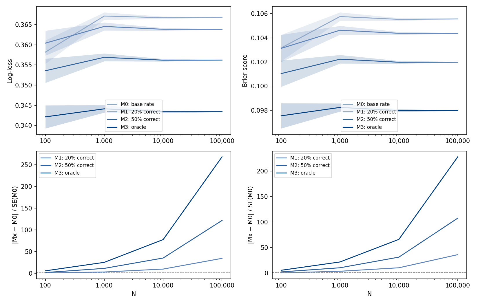
For each size $N\in \{100,1000,10000,100000\}$, generate $500$ datasets of size $N$ such that $95\%$ of the data points are sampled from a $Bernoulli(0.9)$ and the remaining $5\%$ from a $Bernoulli(0.5)$.

We compare the following models:

• M0 (base rate). The base rate predictor, always predicts the average recall of the dataset.
• M1 (20% correct). Predicts 0.9 for reviews generated from $Bernoulli(0.9)$; for reviews generated from $Bernoulli(0.5)$, predicts 0.5 with probability $0.2$ and 0.9 otherwise.
• M2 (50% correct). Predicts 0.9 for reviews generated from $Bernoulli(0.9)$; for reviews generated from $Bernoulli(0.5)$, predicts 0.5 with probability $0.5$ and 0.9 otherwise.
• M3 (oracle). The oracle, predicts 0.9 for reviews generated from $Bernoulli(0.9)$ and 0.5 for reviews generated from $Bernoulli(0.5)$.

For each model and size $N$, we evaluate the mean and standard error for the logloss and Brier score, over the population of $500$ trials. We plot:

• Above: the scores against $N$.
• Below: the ratio $({\bar{S}}_{M0}-{\bar{S}}_{MX})/\text{SE}(M0)$ for each model MX; we interpret this as a signal-to-noise ratio.

As we can see from the plot, for datasets with >100K the signal-to-noise ratio is sufficiently large that both logloss and Brier score are able to distinguish between the base rate predictor and a slightly better model (M1), for better models the signal-to-noise ratio increases. The anki-revlog-10k dataset has over 200M reviews; we conclude that in similar datasets the metrics discussed here can be applied without concern.

Wozniak’s proposed metric works as follows: he uses Algorithm SM-17 as a “classifier” to bin reviews by SM-17’s predicted retrievability into quantiles. Within each bin, he computes the mean prediction-minus-outcome for the algorithm under evaluation, then aggregates these per-bin averages via RMSD. This is essentially measuring calibration (defined formally in the Calibration section below) — whether predicted probabilities match observed frequencies within each bin. Measuring calibration across the full spectrum of predicted retrievability is useful, and this is the strongest aspect of Wozniak’s contribution. However, his metric bins observations using SM-17’s predictions, not those of the model under evaluation. The metric therefore measures alignment with outcomes as partitioned by SM-17, and its verdicts are only as reliable as SM-17’s predictions in each bin.

Finally, the skewed distribution of reviews near retrievability 0.9 does cause real problems, but in model training, not evaluation. Models trained on data overwhelmingly concentrated near retrievability 0.9 can learn to ignore the observations where outcomes diverge from 0.9 — new cards, lapsed items, overdue reviews — while still achieving a low training loss. This kind of degeneracy is a well-known problem in machine learning, addressed through various training-time interventions. The loss function does assign the degenerate model a worse score than a model that makes differentiated predictions; the problem is the optimization process finding a local minimum that corresponds to a degenerate solution, not the appropriateness of the training objective.

That being said, we do want to be able to detect when models fail in this way. We include both a check for temporal collapse and a calibration metric (SmoothECE) in our panel of metrics.

Detecting Temporal Collapse

As already mentioned, temporal collapse is a known failure mode for memory models. However, predicting a flat forgetting curve is not the only way memory models can violate our expectations about how they should behave over time. For example, we’ve observed models predict forgetting curves that go down for a while, then back up!

From the psychological literature, we have a strong prior that, if a memory isn’t recalled, it becomes less and less retrievable over time. If a model doesn’t behave this way, we should be wary. Two possible exceptions are circadian and consolidation effects; respectively, periodic fluctuations over the day, and paradoxical increases in retrievability across sleep boundaries.

Accounting for these, we expect that for any time elapsed since last review $\delta >0$, and forgetting curve $\mu (\delta )$, that:

$$\mu (\delta +1\text{ day})<\mu (\delta )+\epsilon (\delta )$$

where $\epsilon (\delta )\ge 0$ is a tolerance function that is monotonically decreasing and approaches zero.

Unfortunately, this theoretical desideratum is hard to check in practice. Instead, we’re tentatively including an inexpensive sanity check in our panel of evaluations.

Randomly sample $n$ reviews from the validation or test dataset as appropriate and push them through your model to get a sample of ${\mu }_i$. Then, for each ${\mu }_i$, randomly sample $k$ $({\delta }_a,{\delta }_b{)}_j$ pairs from the empirical distribution of intervals from the same dataset and label them such that ${\delta }_a<{\delta }_b$. Finally, simply count the number of the $n\times k$ total samples where $\mu ({\delta }_a)<\mu ({\delta }_b)$ to get a Monte Carlo estimate of the propensity of the model to violate the assumption that it should decrease over time.

We are less confident in this approach than in the other sections of this post; as such, we expect our methodology for evaluating temporal dynamics to change as we learn more.

Calibration

Calibration is a notion rather than a term with a specific consensus definition. When we say calibration we use it to describe a behavioral property of a model. A model is well calibrated if, vaguely, for events the model predicted had probabilities in the neighborhood of $p$, the empirical rate is actually close to $p$.

Specific measures of calibration often differ in how they specify the concept of a neighborhood as used in the prior paragraph, and it is this kind of witting and unwitting decision in the translation of concept to code that makes all the difference to the properties of the resulting measure of “calibration,” so called. It’s worth emphasizing that any measure of model performance is itself a mathematical model which may or may not express what we want.

Side Note: Another thought for future research is the idea that we might want to know the model calibration with respect to neighborhoods of the feature space. This would be feature set specific, and therefore is beyond the scope of this set of metrics focused on general applicability to memory models.

Three Calibration Metrics

Unlike the elegance and clarity of the scoring rules discourse, the study of calibration measures is more confusing. From our reading some principled and popular choices have emerged, but though the theoretical basis for such choices may be there, we are unable to parse all of the theoretical justifications. It’s not so much that there is an absence of proofs, but that, since we don’t understand them ourselves, we won’t simply echo them to you. With that disclaimer, we will introduce SmoothECE, which is the calibration measure we’ve chosen to use.

ECE

The most common approach to measuring calibration is binned Expected Calibration Error (ECE). The idea is straightforward: partition the interval $(0,1)$ into bins — say, $[0,0.1)$, $[0.1,0.2)$, and so on — then, within each bin, compare the average prediction to the fraction of positive outcomes. If the model is well calibrated, predictions averaging $0.25$ within a bin should correspond to roughly 25% positive outcomes in that bin. Binned ECE computes the absolute difference between these two quantities in each bin, then takes a weighted average across bins, weighted by how many predictions fall in each one.

This is intuitive, easy to implement, and easy to visualize — the familiar bar-chart reliability diagram is just a plot of average outcome versus average prediction per bin, and the ECE is the weighted sum of the gaps between the bars and the diagonal. The problem is that the answer depends on the bins. Change the number of bins, or switch from equal-width to equal-mass binning, and the reported calibration error changes — sometimes substantially. A prediction of 0.3001 might land in a different bin than 0.2999, producing a discontinuous jump in the measure for an infinitesimal change in the model. There is no principled basis for choosing 10 bins over 15 or 20, and the choice matters more than practitioners might realize. Variants like RMSE-based binned ECE (which squares the per-bin errors before averaging) share the same fundamental dependence on bin boundaries. The bins are doing real work in determining the answer, and that work is somewhat arbitrary. Moreover, because ECE averages absolute (not signed) differences, sampling noise inside each bin can only inflate the estimate, so a perfectly calibrated model will still report a positive ECE on finite data.

SmoothECE

SmoothECE (Błasiok & Nakkiran, 2024) replaces the bins with kernel smoothing. Instead of asking “among predictions in the bin $[0.25,0.35]$, what fraction of outcomes were positive?”, it asks “among predictions near p, weighted by proximity, what was the average outcome?” The weighting is Gaussian: predictions very close to p contribute heavily, predictions far from p contribute little. This produces a smooth estimate of the calibration function — the function that maps what the model says to what actually happens — without any bin edges to argue about.

The calibration error is then the average absolute gap between this smooth curve and the diagonal (where the curve would be if the model were perfectly calibrated), weighted by where the model’s predictions actually concentrate.

Mechanically, this is something called Nadaraya-Watson kernel regression of outcomes on predictions, followed by integration. It’s a standard ‘nonparametric’ technique.

Kernel smoothing has its own arbitrary choice: the bandwidth σ, which controls how wide the Gaussian weights are. Wide bandwidth → lots of smoothing → you can only see broad miscalibration patterns. Narrow bandwidth → less smoothing → you can see fine structure but also noise.

SmoothECE’s contribution is a specific rule for choosing σ. The rule is: find the value σ* where the reported calibration error equals σ* itself. Because the calibration error decreases monotonically as you increase σ (more smoothing always hides more structure), and σ increases linearly, they cross exactly once. This fixed point is the bandwidth.

The intuition is adaptive resolution: a badly miscalibrated model gets evaluated at coarse resolution (big σ), and a nearly-calibrated model gets a fine-grained evaluation (small σ). The resolution matches the scale of the problem. If you find 5% miscalibration, you were smoothing at roughly 5%. If you find 0.5%, you were smoothing at 0.5%.

We find the mechanical procedure compelling: it avoids bins, it’s continuous, and it removes the most obviously arbitrary choices from the computation. The adaptive bandwidth rule seems reasonable on its face — it avoids under-smoothing (which would find spurious fine-grained miscalibration in finite data) and over-smoothing (which would hide real miscalibration).

The paper proves that the resulting measure is “consistent” in a specific technical sense defined by Błasiok et al. (2023): the smECE value is within a constant factor of the Wasserstein distance from the joint distribution of predictions and outcomes to the nearest perfectly calibrated such distribution. We are not going to pretend we’ve verified these proofs, and the framing involves population-level distributional reasoning that we’re not comfortable with. What we can say is that the measure behaves well empirically, avoids the known pathologies of binned ECE, and we are comfortable trusting the people proving the theorems for now.

Given more time to focus on clarifying calibration measures, we would investigate the fact that the SmoothECE framework is doing something that could be expressed more naturally as a hierarchical Bayesian model: put a flexible prior on the calibration function (say, a spline basis with a shrinkage prior on the coefficients, on the logit scale), fit it to the data, and read off a posterior distribution over calibration error. The bandwidth selection that SmoothECE solves via a fixed-point equation would instead be handled by inference over the smoothness hyperparameter, with uncertainty propagated honestly to the final answer.

We use SmoothECE because we mostly trust the process by which the authors arrived at the conclusion that it’s an improvement over binned ECE approaches, it’s implemented in a clean package (pip install relplot), it produces useful visualizations, and it’s widely used. We flag the Bayesian alternative as future work that we think would be worth doing, if only to further clarify the problem of calibration measurement in language less troubled by map-territory conflation.

Two Calibration Metrics From the Community

We want to address two calibration measures that are already in use in the spaced repetition community. Wozniak’s Universal Metric (discussed earlier) bins reviews by SM-17’s predicted retrievability and computes RMSD of per-bin mean residuals. The FSRS project uses a similar approach: bin reviews by spaced repetition specific features, then compute RMSE of the per-bin calibration gaps.

Both are measuring something real — they ask whether predicted probabilities match observed frequencies across the range of predictions, which is exactly the question calibration metrics should answer. We don’t claim these measures are wrong, and for the practical purpose of iterating on a model during development, they clearly work: the FSRS team has used their RMSE bins metric to successfully guide improvements over several model versions.

However, both metrics inherit the problems with binning described above: dependence on the number and placement of bin edges, discontinuity at bin boundaries, and sensitivity to the binning scheme. Additionally, both use model-dependent binning — the Universal Metric bins by SM-17’s predictions, and the FSRS metric bins by spaced repetition specific features — which can be thought of as a model in itself. This means the partition of the data changes when you change the model, which makes it harder to reason about what a change in the metric actually reflects: did the model’s calibration improve, or did the new predictions just land in the bins differently? We haven’t carried out a formal analysis of the consequences of model-dependent binning, but our intuition is that it introduces coupling between the measure and the thing being measured that will be harder to reason about as models become more complex.

We don’t have a strong argument that these concerns matter in practice for current spaced repetition models. What we do have is a measure — SmoothECE — that avoids them entirely, is theoretically grounded, and is easy to compute. Given the choice between a binned metric we feel has more foot-gun potential and a widely used tool specifically designed to avoid the binning issues, supported by epistemologically trustworthy parties, we prefer the latter. If future work (ours or others’) demonstrates that SmoothECE and the community metrics disagree in ways that matter, our choice now should be re-questioned to see if it’s still reasonable given all the evidence practically available.

Discrimination

Discrimination is the model’s ability to distinguish reviews where the student will recall the card from reviews where they won’t. Unlike scoring rules and calibration, which evaluate the model as a probabilistic forecaster, measures of discrimination treat the model as a binary classifier: it predicts the student will recall, or that they won’t recall.

Since a memory model outputs a probability $p\in (0,1)$ for each review, we must impose some threshold $\tau$ on all model outputs, predicting “will recall” if $p\ge \tau$ and “won’t recall” if $p<\tau$. Different choices for $\tau$ produce different classifiers from the same memory model. Discrimination metrics characterize how well the model separates the two classes across the full range of possible thresholds, or a particular threshold of interest.

The Confusion Matrix

For a given threshold $\tau$, every review falls into one of four categories:

	Actually recalled $(y=1)$	Actually forgot $(y=0)$
Predicted recall $(p\ge \tau )$	True Positive (TP)	False Positive (FP)
Predicted forgot $(p<\tau )$	False Negative (FN)	True Negative (TN)

We call this a confusion matrix. From it we derive several useful rates. Actually there are 8 empirical conditional probabilities you probably care about.

Model predictions, conditioned on student outcomes:

• $P(\text{Model Predicted Recall}|\text{Student Actually Recalled})$ = True Positive Rate aka Sensitivity
• $P(\text{Model Predicted Recall}|\text{Student Actually Forgot})$ = False Positive Rate
• $P(\text{Model Predicted Forgetting}|\text{Student Actually Recalled})$ = False Negative Rate
• $P(\text{Model Predicted Forgetting}|\text{Student Actually Forgot})$ = True Negative Rate aka Specificity

Student outcomes, conditioned on model predictions:

• $P(\text{Student Actually Recalled}|\text{Model Predicted Recall})$ = Precision aka Positive Predictive Value
• $P(\text{Student Actually Recalled}|\text{Model Predicted Forgetting})$ = False Omission Rate
• $P(\text{Student Actually Forgot}|\text{Model Predicted Recall})$ = False Discovery Rate
• $P(\text{Student Actually Forgot}|\text{Model Predicted Forgetting})$ = Negative Predictive Value

We will refer to the 8 above probabilities as the Confusion Statistics.

Side Note: You may encounter the terms “type 1 error” and “type 2 error” in discussions of binary classification. These mean, respectively, falsely detecting a problem that isn’t there, and failing to detect a problem that is. We mention this only so you can translate if you encounter these terms elsewhere. We won’t use them ourselves.

The Receiver Operating Characteristic (ROC) and the Area Under Its Curve (AUC)

The Receiver Operating Characteristic (ROC) curve traces out the tradeoff between the True Positive Rate (TPR) and the False Positive Rate (FPR) as the threshold $\tau$ sweeps from 1 down to 0. At $\tau =1$, the model predicts “forgot” for everything: $\text{TPR}=0$, $\text{FPR}=0$. At $\tau =0$, the model predicts “recall” for everything: $\text{TPR}=1$, $\text{FPR}=1$. In between, as the threshold decreases, both TPR and FPR increase, tracing a curve from $(0,0)$ to $(1,1)$.

A model with no discriminative ability — one whose predictions are independent of the outcomes — traces the diagonal from $(0,0)$ to $(1,1)$. A model with perfect discrimination traces the upper-left corner: it can achieve $\text{TPR}=1$ with $\text{FPR}=0$ at some threshold. Most models fall somewhere in between, bowing above the diagonal.

The Area Under the ROC Curve (AUC) summarizes this curve as a single number between 0 and 1. An AUC of 0.5 means no discrimination (the diagonal). An AUC of 1.0 means perfect discrimination. The AUC has a probabilistic interpretation: if you randomly draw one review where the student recalled and one where they forgot, the AUC gives the probability that the model assigned a higher retrievability to the recalled review. This is equivalent to saying the AUC measures how well the model ranks reviews by recall probability. But ranking is all it measures. A model that predicts 0.51 for every recall and 0.49 for every lapse achieves AUC = 1.0 — perfect discrimination — while being nearly useless as a probabilistic forecast. The predicted probabilities are wrong for almost every review, but they are in the right order. This is why AUC alone is insufficient for evaluating memory models: we need the probabilities themselves to be correct. The proper scoring rules and calibration metrics fill that gap.

Reporting The Confusion Statistics at $\tau \in \{0.85,0.9,0.95\}$

The AUC and ROC curve summarize discrimination across all thresholds, but in practice a spaced repetition user cares about specific retrievability targets. A student who wants to maintain 90% recall is operating at $\tau =0.9$. We report all 8 confusion statistics at $\tau \in \{0.85,0.9,0.95\}$, since these are the retrievability levels a user is most likely to care about. Popular SRS apps like Anki and RemNote default to 90% desired retention. This gives a concrete picture of model behavior at the thresholds that actually matter: how often does the model correctly identify cards that will be forgotten, how often does it raise false alarms, and so on — at the specific operating points a scheduler would use.

There is a deeper reason to evaluate at specific thresholds beyond user preference. When a scheduler thresholds a memory model’s output at some $\tau$, the scheduling decision is sensitive to small systematic biases in the model’s predictions near $\tau$. These biases may not be apparent in aggregate metrics — a model can have excellent overall calibration and discrimination while being systematically biased in the narrow region around 0.9 where the scheduler actually operates. Reporting the confusion statistics at the thresholds the scheduler will use detects exactly this kind of failure.

Conclusion

Our evaluation panel consists of six components: normalized entropy, Brier skill score, SmoothECE (with calibration plot), AUC (with ROC curve), the 8 confusion statistics at $\tau \in \{0.85,0.9,0.95\}$, and a temporal discrimination check. No single metric tells the whole story. The proper scoring rules measure overall predictive quality. SmoothECE checks whether the model’s probabilities mean what they say. AUC and the confusion statistics assess the model’s ability to distinguish recalls from lapses. The temporal check catches models that have given up on modeling forgetting altogether.

We have tried to be careful throughout this post about the distinction between what we compute from data — averages of scores over predictions and outcomes — and the distributional concepts that are often invoked to justify those computations. The metrics we report are all functions of predictions and outcomes. They do not require positing a true data distribution, and we think the field is better served by keeping that clear.

This panel is not final. As we learn more about what matters in practice for spaced repetition, we expect it to evolve — particularly around calibration measurement and temporal dynamics, where we are least confident in our current choices.

References and Further Reading

Scoring Rules. For a clear introduction to scoring rules, we recommend the above quoted blog post by Sebastian Nowozin. Proper Scoring Rules for Estimation and Forecast Evaluation by Bálint Mucsányi et al. is a more thorough treatment, covering a wider family of scoring rules and their properties.

Brier Score. Brier, G. W. (1950). Verification of Forecasts Expressed in Terms of Probability. Monthly Weather Review, 78(1), 1–3. The original paper introducing the Brier score in the context of weather forecasting.

Calibration of Neural Networks. Guo et al. (2017). On Calibration of Modern Neural Networks. ICML 2017. Demonstrates that modern neural networks can achieve excellent predictive accuracy while being poorly calibrated — their predicted confidences don’t match observed frequencies. Established ECE as the standard calibration metric in deep learning and introduced temperature scaling as a simple post-hoc fix.

Problems with Binned ECE. The following three papers document specific failures of binned ECE that motivated our choice of SmoothECE:

• Roelofs et al. (2022). Mitigating Bias in Calibration Error Estimation. AISTATS 2022. Shows that binned ECE has a systematic positive bias for well-calibrated models — finite-sample noise inflates the estimate even when calibration is perfect, and this bias can reverse model rankings.
• Kumar et al. (2019). Verified Uncertainty Calibration. NeurIPS 2019. Proves that ECE with a fixed number of bins is inconsistent: it systematically underestimates true calibration error even in the infinite-data limit.
• Nixon et al. (2019). Measuring Calibration in Deep Learning. CVPR 2019 Workshop. Shows that changing the number of bins or the binning scheme can flip which model appears better calibrated.

Theoretical Foundations for SmoothECE. Błasiok et al. (2023). A Unifying Theory of Distance from Calibration. STOC 2023. Proves that ECE is not a consistent calibration measure and establishes the theoretical framework underlying SmoothECE. The applied version is Błasiok & Nakkiran (2024), Smooth ECE: Principled Reliability Diagrams via Kernel Smoothing, which implements the theory as a practical tool (pip install relplot).

ML Calibration vs. Decision-Making Calibration. Hartline (2025). Smooth Calibration and Decision Making. FORC 2025. Formalizes the distinction between two types of calibration: smooth calibration (continuous in prediction space, appropriate for evaluating probability estimates) and decision-making calibration (discontinuous, measuring whether thresholding at specific boundaries produces correct decisions). The central result — that low smooth calibration error does not guarantee low decision-making calibration error — is directly relevant to why we report confusion statistics at specific thresholds in addition to SmoothECE.

Memory Models for Spaced Repetition Systems. Giacomo’s Master’s thesis at Politecnico di Milano. Introduces and compares several memory models for spaced repetition, including DASH[RNN] and R-17, evaluated on real-world review data. A useful starting point for readers wanting background on the models this evaluation framework is designed to compare.

SRS Benchmark. The FSRS team’s SRS Benchmark provides open-source tooling for comparing spaced repetition algorithms on real datasets.